PCA - Principal Component Analysis
PCA
Prerequisites
1
2
3
eigenvector
eigenvalue
eigen decomposition
What is PCA
1. What is PCA?
Principle Component Analysis(PCA) is a technique used to find the directions in which data variance the most
Variance is proportional to information. when we want to compress the capacity of files or reduce dimensions, we choose the part of dimension. And if we want to get similar quality but compress the size, we should find the dimension of condensed data information.
The more eigenvalue is large number, the more information remain. So that’s why we use the PCA method.
- Identify the principal directions of variance
- Represent the data in a new coordinate system
- Optionally reduce dimensionality
PCA finds the directions of maximum variance where the data spreads the most.
Where the method use?
- Dimensionality reduction
- Noise filtering
- Feature extraction
- Data visualization
- Image compression
- Face recognition (Eigenfaces)
- Data preprocessing for machine learning
2. How to calculate PCA.
1
Data → Centering with mean → Covariance Matrix → Eigen Decomposition
Assume we have a dataset:
\[X = \begin{bmatrix} x_{11} & x_{12} & \cdots & x_{1d} \\ x_{21} & x_{22} & \cdots & x_{2d} \\ \vdots & \vdots & \ddots & \vdots \\ x_{n1} & x_{n2} & \cdots & x_{nd} \end{bmatrix}\]Where:
- Rows = data samples
- Columns = features
1. Mean Centering
Before applying PCA, the data is centered by subtracting the mean.
\[X_c = X - \mu\]This ensures the dataset is centered around the origin.
PCA analyzes the variance structure of the data.
2. Covariance Matrix
The covariance matrix captures how features vary together.
\[C = \frac{1}{n} X_c^T X_c\]For two features, the covariance matrix looks like:
\[C = \begin{bmatrix} \text{Var}(x) & \text{Cov}(x,y) \\ \text{Cov}(x,y) & \text{Var}(y) \end{bmatrix}\]Meaning:
- Variance measures spread along a single feature
- Covariance measures how two features change together
3. Eigen Decomposition
Next, compute the eigenvectors and eigenvalues of the covariance matrix.
\[Cv = \lambda v\]Where:
- $v$ = eigenvector
- $\lambda$ = eigenvalue
Interpretation:
| Quantity | Meaning |
|---|---|
| Eigenvector | Direction of maximum variance |
| Eigenvalue | Amount of variance in that direction |
4. Principal Components
The eigenvectors sorted by largest eigenvalue define the principal components.
- PC1 → direction with largest variance
- PC2 → second largest variance
- etc.
These vectors form a new coordinate system.
5. Projection onto Principal Components
To express the data in the new coordinate system:
\[Z = X_c V\]Where:
- $V$ = matrix of eigenvectors
If we keep only the first $k$ components:
\[Z_k = X_c V_k\]This performs dimensionality reduction.
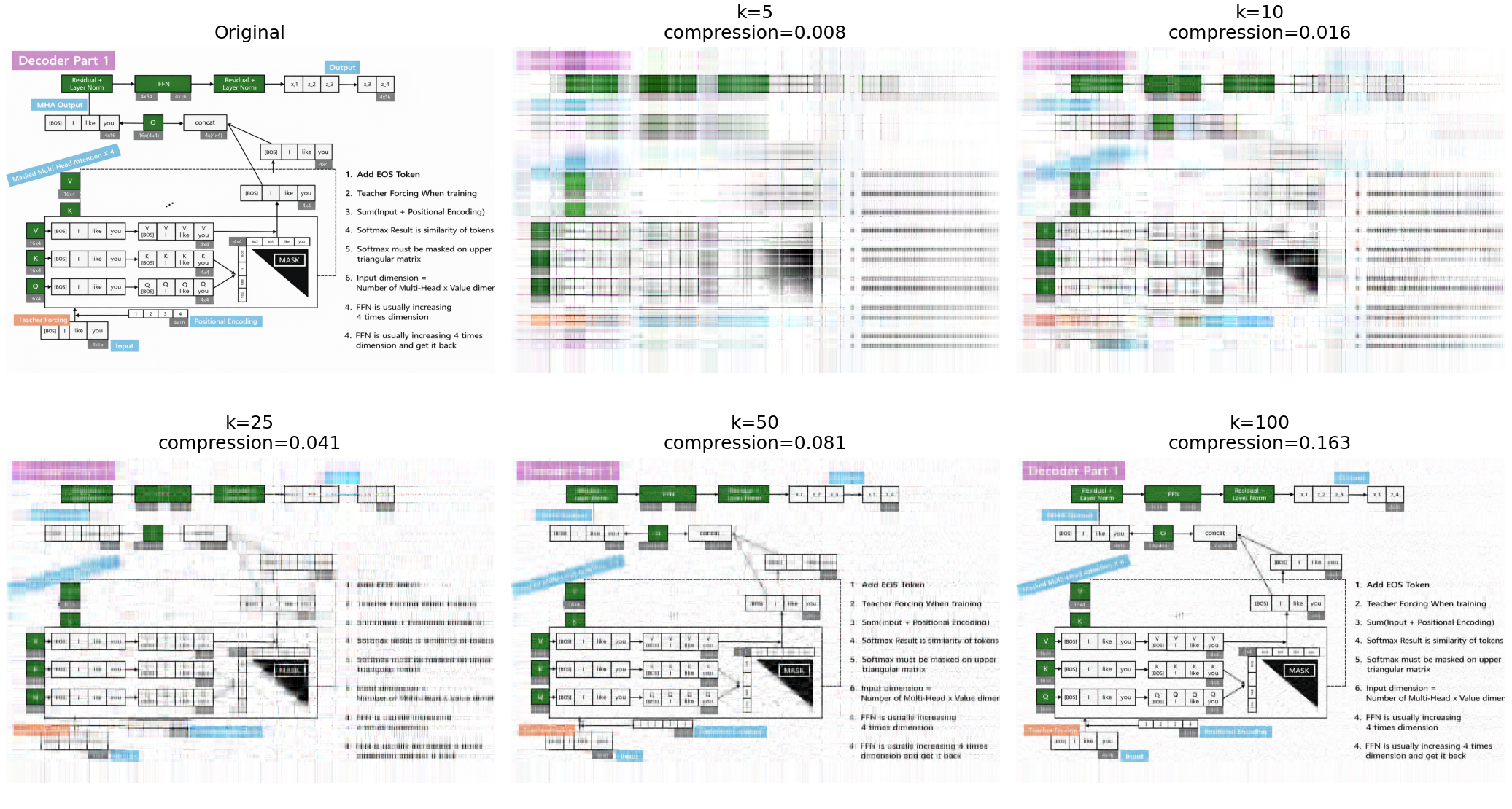
3. PCA Example
The example image rank is 1024.
Let’s see the PCA result.