SVD - Singular Value Decomposition

SVD

---

Prerequisites

eigenvector
eigenvalue
eigen decomposition

---

What is SVD

1. What is PCA?

Singular Value Decomposition (SVD) is a fundamental matrix factorization technique in linear algebra.

For any real matrix

\[X \in \mathbb{R}^{m \times n}\]

SVD factorizes the matrix into three components:

\[X = U \Sigma V^T\]

Where:

• $U \in \mathbb{R}^{m \times m}$ → left singular vectors
• $\Sigma \in \mathbb{R}^{m \times n}$ → diagonal matrix of singular values
• $V \in \mathbb{R}^{n \times n}$ → right singular vectors

---

2. Matrix Structure

The decomposition can be written as:

\[X = U \begin{bmatrix} \sigma_1 & 0 & \cdots & 0 \\ 0 & \sigma_2 & \cdots & 0 \\ \vdots & \vdots & \ddots & \vdots \\ 0 & 0 & \cdots & \sigma_r \end{bmatrix} V^T\]

Where:

• $r = \text{rank}(X)$
• $\sigma_1 \ge \sigma_2 \ge \dots \ge \sigma_r \ge 0$

These values are called singular values.

Orthogonality

The matrices $U$ and $V$ are orthogonal:

\[U^T U = I\] \[V^T V = I\]

Singular Values

The singular values are related to eigenvalues:

\[X^T X = V \Sigma^2 V^T\] \[X X^T = U \Sigma^2 U^T\]

Thus:

• columns of $V$ are eigenvectors of $X^T X$
• columns of $U$ are eigenvectors of $X X^T$

---

3. Geometric Interpretation

SVD describes a linear transformation as three steps:

1. Rotation $by (V^T)$ : Input space rotation
2. Scaling $by (\Sigma)$ : Input space to output space with scaling
3. Rotation $by (U)$ : Output space rotation

So any matrix transformation can be interpreted as rotate → scale → rotate

Why $V$ and $U$ is rotation?

\[Q^T Q = I\]

Taking determinants on both sides:

\[\det(Q^T Q) = \det(I)\]

Using determinant properties:

\[\det(Q^T)\det(Q) = 1 \quad \rightarrow \quad \det(Q^T) = \det(Q) \quad \rightarrow \quad \det(Q)^2 = 1\]

Therefore:

\[\det(Q) = \pm 1\]

---

4. Low-Rank Approximation

SVD allows approximation of a matrix using fewer components.

Using only the first (k) singular values:

\[X_k = U_k \Sigma_k V_k^T\]

Where:

• $U_k \in \mathbb{R}^{m \times k}$
• $\Sigma_k \in \mathbb{R}^{k \times k}$
• $V_k \in \mathbb{R}^{n \times k}$

This gives the best rank-(k) approximation of (X).

5. Numerical Example

\[X = U \Sigma V^T\] \[X = \begin{bmatrix} 3 & 1 \\ 0 & 2 \end{bmatrix}\]

$ X^T X = \begin{bmatrix} 9 & 3
3 & 5 \end{bmatrix} $

Singular Values

$ \det(X^T X - \lambda I) = 0 \quad \rightarrow \quad \lambda_1 = 10, \quad \lambda_2 = 4 $

\[\Sigma = \begin{bmatrix} \sqrt{10} & 0 \\ 0 & 2 \end{bmatrix}\]

Compute $V$

Eigenvectors of $X^T X$ form the matrix $V$.

$ \lambda_1 = 10 \quad \rightarrow \quad v_1 = \begin{bmatrix} 0.89
0.45 \end{bmatrix} $

$ \lambda_2 = 4 \quad \rightarrow \quad v_2 = \begin{bmatrix} -0.45
0.89 \end{bmatrix} $

\[V = \begin{bmatrix} 0.89 & -0.45 \\ 0.45 & 0.89 \end{bmatrix}\]

Compute $U$

$ U = X V \Sigma^{-1} $

\[U \approx \begin{bmatrix} 0.96 & -0.28 \\ 0.28 & 0.96 \end{bmatrix}\]

Result

\[X = \begin{bmatrix} 0.96 & -0.28 \\ 0.28 & 0.96 \end{bmatrix} \begin{bmatrix} \sqrt{10} & 0 \\ 0 & 2 \end{bmatrix} \begin{bmatrix} 0.89 & 0.45 \\ -0.45 & 0.89 \end{bmatrix}\]

6. Image Compression Example

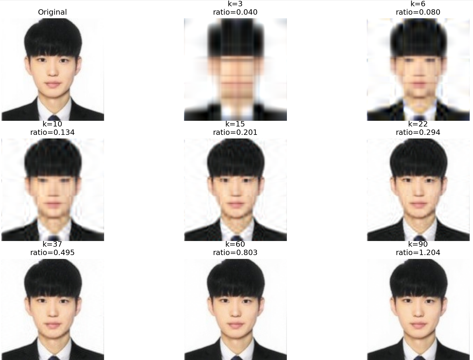
We can see the compression ratio of depending on rank selected. Even though there’re low memory for image, but the quality is not too bad. The compression ratio is sometimes over 1.0 because it is difference format for saving.

Original Image

\[\text{Original storage} = HW\]

Using SVD:

\[X \approx U_k \Sigma_k V_k^T\]

Where: $U_k \in \mathbb{R}^{H \times k}$, $\Sigma_k \in \mathbb{R}^{k \times k}$, $V_k^T \in \mathbb{R}^{k \times W}$

The number of stored values becomes:

\[\text{Compressed storage} = Hk + kW + k\]

The compression ratio is estimated as

\[\text{Compression Ratio} = \frac{Hk + kW + k}{HW}\]