01. Multi-layer Perceptrons

---

Multi-layer Perceptrons

---

Prerequisites

1. Linear Classifiers <b>Linear Classifiers</b> $ f(x) = Wx $ have a problem that <span style="color:#FFD5D5">FAILS on NON-LINEAR SEPERABLE DATA</span>. 

---

What is Multi-Layer Perceptrons

1. What is Multi-layer Perceptrons(MLP)?

• A Feedforward Neural Network composed of multiple fully connected layers with nonlinear activation functions.

• Structure

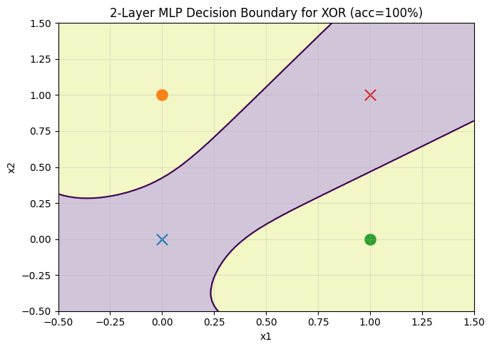
  \[Input \rightarrow FC \rightarrow Activation \rightarrow FC ... \rightarrow Softmax \rightarrow Output\]

• Can express non-linear seperable data like XOR

2. Why use Multi-layer Perceptrons(MLP)?

 Linear/Non-Linear Seperable Data

About Single Perceptron

\[y = f(w_1x_1+w_2x_2), \:\:\:\:\:\:\:\ \text{f}(x) = \begin{cases} 1, & x > 0 \\ 0, & \le 0 \end{cases}\]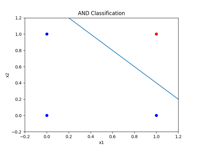

| x1 | x2 | y | |----|----|---| | 0 | 0 | 0 | | 0 | 1 | 0 | | 1 | 0 | 0 | | 1 | 1 | 1 |

Seperating is POSSIBLE on linear data.

| x1 | x2 | y | |----|----|---| | 0 | 0 | 0 | | 0 | 1 | 1 | | 1 | 0 | 1 | | 1 | 1 | 0 |

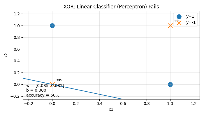
Seperating is IMPOSSIBLE on non-linear data.

BUT Change From Single to Multi-layer, it is POSSIBLE.

\[y = f(w_5f(w_1x_1+w_2x_2) + w_6f(w_3x_1+w_4x_2))\] \[h = \sigma(W_1 x), \quad y = W_2 h\]

3. How use Multi-layer Perceptrons(MLP)?

Fully-Connected Layer $$\mathbf{y} = W\mathbf{x} + \mathbf{b}$$

• $ \mathbf{x} \in \mathbb{R}^{n} $ : input vector
• $ W \in \mathbb{R}^{m \times n} $ : weight matrix
• $ \mathbf{b} \in \mathbb{R}^{m} $ : bias vector
• $ \mathbf{y} \in \mathbb{R}^{m} $ : output vector

Affine transformation on the input vector, where every input neuron is connected to every output neuron.

\[y_i = \sum_{j=1}^{n} w_{ij} x_j + b_i\]

Each output unit is connected to all input units.

Concept of Space Transformation:

An FC layer linearly transforms the input feature space into another space:

\[\mathbf{x} \rightarrow \text{feature transformation} \rightarrow \mathbf{y}\]

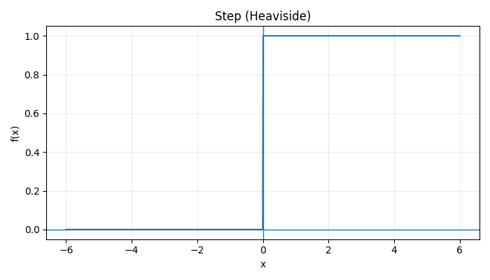
Acitivation Functions

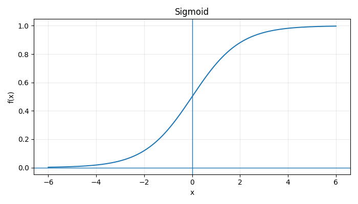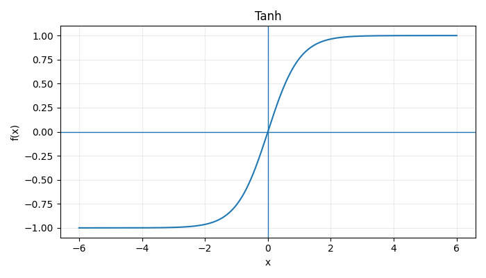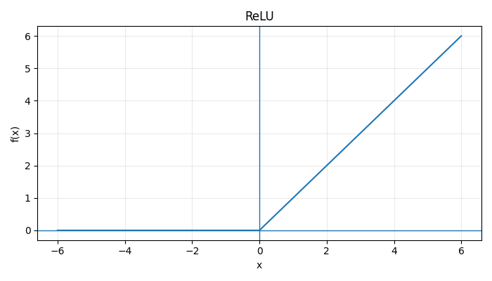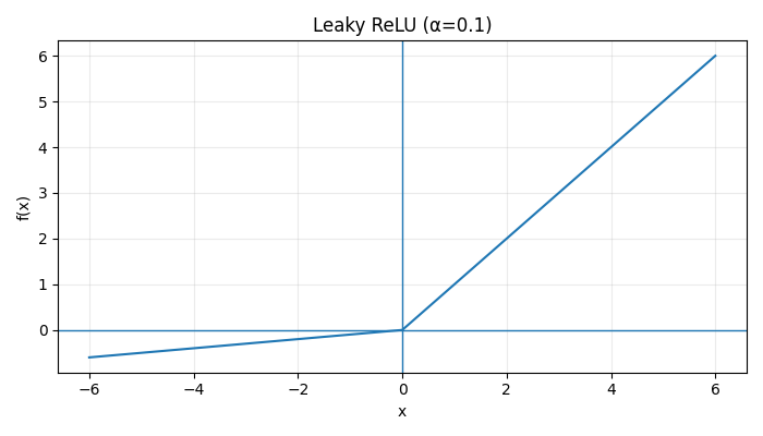\(\text{Step}(x) = \begin{cases} 1, & x \ge 0 \\ 0, & x < 0 \end{cases} \:\:\:\: \sigma(x) = \frac{1}{1 + e^{-x}} \:\:\:\: \tanh(x) = \frac{e^x - e^{-x}}{e^x + e^{-x}}\) \(\text{ReLU}(x) = \max(0, x)\) $$ \text{LeakyReLU}(x) = \begin{cases} x, & x > 0
\alpha x, & x \le 0 \end{cases}

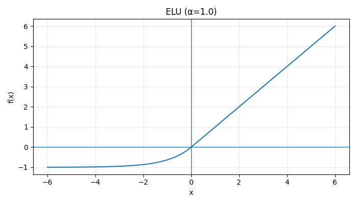
:::: \text{ELU}(x) = \begin{cases} x, & x > 0
\alpha (e^x - 1), & x \le 0 \end{cases} $$

Backpropagation

The main target of backpropgation is Minimize Loss Functions.

Function Example:

\[\hat{y} = W_2 \sigma(W_1 \mathbf{x} + \mathbf{b}_1) + b_2\]

Loss(MSE):

\(L = (\hat{y} - y)^2\)

Backpropagation Derivation

---

\[\hat{y} = W_2 \mathbf{h}, \quad \frac{\partial L}{\partial \hat{y}} = 2(\hat{y} - y), \quad \frac{\partial \hat{y}}{\partial W_2} = \mathbf{h}\] \[\boxed{ \frac{\partial L}{\partial W_2} ===== \frac{\partial L}{\partial \hat{y}} \frac{\partial \hat{y}}{\partial W_2} ===== 2(\hat{y} - y)\mathbf{h} }\] \[\boxed{ \frac{\partial L}{\partial \mathbf{h}} ===== \frac{\partial L}{\partial \hat{y}} \frac{\partial \hat{y}}{\partial \mathbf{h}} ===== 2(\hat{y}-y) W_2 }\]

---

\[\mathbf{z}_1 = W_1 \mathbf{x}, \quad \frac{\partial \mathbf{z}_1}{\partial W_1} = \mathbf{x}\]

If sigmoid:

\[\sigma'(z) = \sigma(z)(1-\sigma(z))\] \[\boxed{ \frac{\partial L}{\partial \mathbf{z}_1} ===== \frac{\partial L}{\partial \mathbf{h}} \odot \sigma'(\mathbf{z}_1) ===== 2(\hat{y}-y) W_2 \odot \mathbf{h}(1-\mathbf{h}) }\] \[\boxed{ \frac{\partial L}{\partial W_1} ===== \frac{\partial L}{\partial \mathbf{z}_1} \mathbf{x}^T }\]

Final:

\[\boxed{ \frac{\partial L}{\partial W_1} ================ 2(\hat{y}-y) W_2 \odot \mathbf{h}(1-\mathbf{h}) \mathbf{x}^T }\]

🔥 Core Idea

Forward:

\[\mathbf{x} \rightarrow \mathbf{z} \rightarrow \mathbf{a} \rightarrow \hat{y}\]

Backward:

\[\frac{\partial L}{\partial \mathbf{x}} ==== \frac{\partial L}{\partial \mathbf{a}} \frac{\partial a}{\partial \mathbf{z}} \frac{\partial \mathbf{z}}{\partial \mathbf{x}} ==== \frac{\partial L}{\partial \mathbf{z}} \frac{\partial \mathbf{z}}{\partial \mathbf{x}}\]

Backpropagation = Chain Rule applied in reverse order.