Hands-on 07. SHAP
SHAP
Prerequisites
1
SHAP
1. How to implement the real
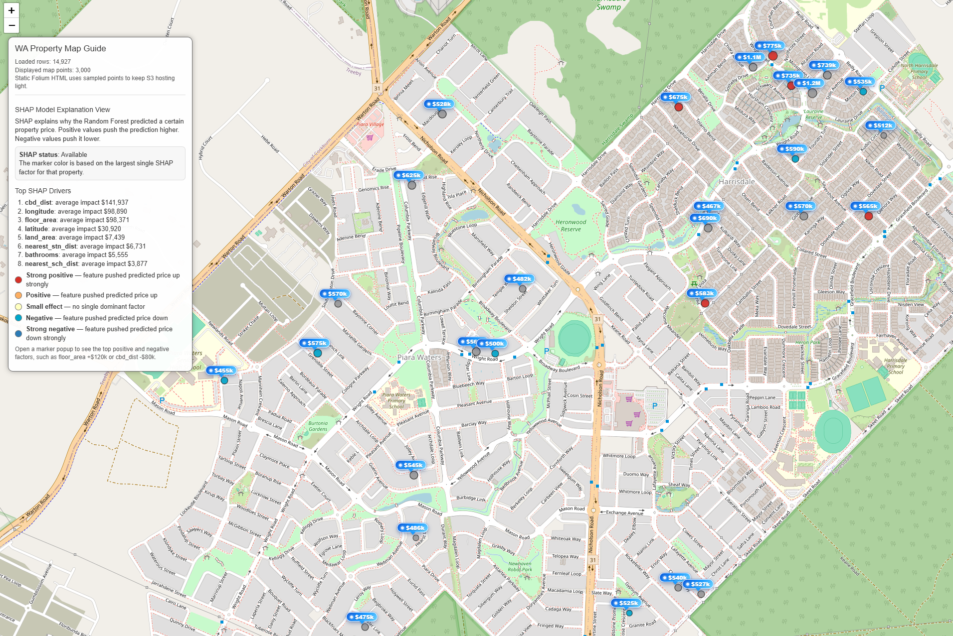
SHAP is a model interpretation algorithm.
The main idea is:
1
2
Measure how much each feature contributed
to the final prediction.
In other words:
1
2
3
Base prediction
+ feature contributions
= final prediction
1
2
3
4
5
6
7
8
9
10
11
12
13
14
15
16
17
18
19
20
21
22
23
24
25
26
27
28
29
30
31
32
33
34
35
36
37
38
39
40
41
42
43
44
45
46
47
48
49
50
51
52
53
54
55
56
57
58
59
60
61
62
63
64
65
66
67
68
69
70
71
72
73
74
75
76
77
78
79
80
81
82
83
84
85
86
87
88
89
90
91
92
93
94
95
96
97
98
99
100
101
102
103
104
105
106
107
108
109
110
111
112
113
114
115
116
117
118
119
120
121
122
123
124
125
126
127
128
129
130
131
132
133
134
135
136
137
138
139
140
141
142
143
144
145
146
147
148
149
150
151
152
153
154
155
156
157
from sklearn.ensemble import RandomForestRegressor
import shap
import numpy as np
import pandas as pd

model_df = pd.DataFrame({
    "bedrooms": [3, 4, 3, 5, 4],
    "bathrooms": [2, 2, 1, 3, 2],
    "land_area": [500, 650, 420, 800, 700],
    "floor_area": [180, 240, 130, 320, 260],
    "cbd_dist": [12, 8, 20, 6, 10],
    "nearest_stn_dist": [1.2, 0.8, 2.5, 0.6, 1.0],
    "price": [720000, 950000, 560000, 1250000, 1050000],
})

RANDOM_STATE = 42
MAX_SHAP_EXPLANATION_ROWS = 1000

def money_effect(value):
    sign = "+" if value >= 0 else "-"
    return f"{sign}${abs(value):,.0f}"

available_features = [
    "bedrooms",
    "bathrooms",
    "land_area",
    "floor_area",
    "cbd_dist",
    "nearest_stn_dist",
]

X = model_df[available_features]
y = model_df["price"]

# Random Forest Training
model = RandomForestRegressor(
    n_estimators=100,
    max_depth=5,
    random_state=RANDOM_STATE,
)

model.fit(X, y)
model_df["predicted_price"] = model.predict(X)

#-----------------------------------------------------#

if len(model_df) > MAX_SHAP_EXPLANATION_ROWS:
    shap_index = model_df.sample(
        n=MAX_SHAP_EXPLANATION_ROWS,
        random_state=RANDOM_STATE,
    ).index
else:
    shap_index = model_df.index

X_shap = X.loc[shap_index]

explainer = shap.TreeExplainer(model) # SHAP for tree structure
shap_values = explainer.shap_values(X_shap) # features effect using SHAP
{
    if isinstance(shap_values, list):
        shap_values = shap_values[0]

    shap_values = np.asarray(shap_values)
}

mean_abs = np.abs(shap_values).mean(axis=0)

base_value = explainer.expected_value # base value of SHAP
{
    if isinstance(base_value, (list, np.ndarray)):
        base_value = float(np.asarray(base_value).ravel()[0])
    else:
        base_value = float(base_value)
}

shap_summary_features = sorted(
    zip(available_features, mean_abs),
    key=lambda x: x[1],
    reverse=True,
)[:8]

shap_summary_features = [
    (name, float(value))
    for name, value in shap_summary_features
]

shap_result = pd.DataFrame(index=shap_index)

shap_result["shap_base_value"] = base_value
shap_result["shap_total_effect"] = shap_values.sum(axis=1)
shap_result["shap_top_positive"] = "N/A"
shap_result["shap_top_negative"] = "N/A"
shap_result["shap_explanation"] = "N/A"
shap_result["shap_dominant_feature"] = "N/A"
shap_result["shap_dominant_value"] = np.nan

for row_pos, idx in enumerate(shap_index):

    vals = shap_values[row_pos]

    pairs = list(zip(available_features, vals))

    pos = sorted(
        [p for p in pairs if p[1] > 0],
        key=lambda x: x[1],
        reverse=True,
    )[:3]

    neg = sorted(
        [p for p in pairs if p[1] < 0],
        key=lambda x: x[1],
    )[:3]

    dominant = max(
        pairs,
        key=lambda x: abs(x[1]),
    )

    pos_text = (
        "; ".join(
            [f"{name}: {money_effect(value)}" for name, value in pos]
        )
        if pos
        else "None"
    )

    neg_text = (
        "; ".join(
            [f"{name}: {money_effect(value)}" for name, value in neg]
        )
        if neg
        else "None"
    )

    explanation = (
        f"Base price: ${base_value:,.0f}<br>"
        f"Positive factors: {pos_text}<br>"
        f"Negative factors: {neg_text}"
    )

    shap_result.loc[idx, "shap_top_positive"] = pos_text
    shap_result.loc[idx, "shap_top_negative"] = neg_text
    shap_result.loc[idx, "shap_explanation"] = explanation
    shap_result.loc[idx, "shap_dominant_feature"] = dominant[0]
    shap_result.loc[idx, "shap_dominant_value"] = float(dominant[1])

shap_cols = [
    "shap_base_value",
    "shap_total_effect",
    "shap_top_positive",
    "shap_top_negative",
    "shap_explanation",
    "shap_dominant_feature",
    "shap_dominant_value",
]

model_df.loc[shap_result.index, shap_cols] = shap_result[shap_cols]
1-1. Data
Set parameters
- Trained tree model (Random Forest / XGBoost / LightGBM)
- Input data to explain
- Feature list
- Background / base prediction
- Maximum rows for SHAP calculation
1-2. SHAP Model
Process as follows:
Create a TreeExplainer
Pass the trained tree model to SHAP
1
explainer = shap.TreeExplainer(model)
SHAP reads the tree structure:
- Split features
- Split thresholds
- Leaf prediction values
- Tree paths
Select data to explain
- If the dataset is large, sample only part of it
- This reduces computation time
1
X_shap = X.loc[shap_index]
Compute base value
- Base value means the model’s average expected prediction
- It is the starting point before feature effects are added
1
base_value = explainer.expected_value
Example:
1
Base value = 650k
Compute SHAP values
- For each row, SHAP calculates how much each feature moves the prediction
- Positive value → pushes prediction higher
- Negative value → pushes prediction lower
1
shap_values = explainer.shap_values(X_shap)
Explain one prediction
Example:
1
2
3
4
5
6
Base value = 650k

floor_area = +150k
cbd_dist   = +100k

Final prediction = 900k
Calculation:
1
650k + 150k + 100k = 900k
Repeat for all rows
- For every house, SHAP calculates feature contribution values
Example:
1
2
3
4
5
6
7
House A:
floor_area = +120k
cbd_dist   = +80k

House B:
floor_area = -60k
cbd_dist   = -100k
Aggregate feature importance
- Compute average absolute SHAP value for each feature
- Larger average absolute value means stronger overall model influence
1
mean_abs = np.abs(shap_values).mean(axis=0)
Example:
1
2
3
cbd_dist   = 140k average impact
floor_area = 120k average impact
bathrooms  = 20k average impact
Determine dominant feature
- For each row, find the feature with the largest absolute SHAP value
1
dominant = max(pairs, key=lambda x: abs(x[1]))
Example:
1
2
3
4
floor_area = +150k
cbd_dist   = +100k

Dominant feature = floor_area
Final output
- Base value
- SHAP values for each feature
- Positive factors
- Negative factors
- Dominant feature
- Feature importance summary
Example:
1
2
3
4
5
6
7
8
9
10
11
Base price: 650k

Positive factors:
floor_area: +150k
cbd_dist: +100k

Negative factors:
None

Final prediction:
900k
Core rule
1
2
3
4
5
Final prediction
=
Base value
+
Sum of SHAP values
Interpretation
- Positive SHAP value → feature increased the prediction
- Negative SHAP value → feature decreased the prediction
- Large absolute SHAP value → feature had strong influence
- Small absolute SHAP value → feature had weak influence
1.2 In real
2. How to work Random Forest
Example Data
Assume we trained a Random Forest model using:
1
2
3
4
price
floor_area
cbd_dist
bathrooms
We want to predict:
1
2
3
4
House E:
floor_area = 250
cbd_dist = 8
bathrooms = 2
Suppose the Random Forest predicts:
1
Predicted price = 900k
Now SHAP asks:
1
Why did the model predict 900k?
2-1. Base Value
SHAP first calculates the average prediction of the model.
Example:
1
Average house prediction = 650k
This becomes:
1
base_value = 650k
Meaning:
1
2
Without knowing any feature,
the model predicts around 650k.
2-2. Tree Contribution Calculation
Suppose one decision tree looks like:
1
2
3
4
5
6
7
8
9
                [floor_area < 200]

                 /             \
              YES               NO
           predict 500k      [cbd_dist < 10]

                              /          \
                           YES            NO
                        predict 900k   predict 700k
Our house:
1
2
floor_area = 250
cbd_dist = 8
Step 1
1
floor_area < 200 ?
Result:
1
2
250 > 200
→ NO
Move right.
Step 2
1
cbd_dist < 10 ?
Result:
1
2
8 < 10
→ YES
Final prediction:
1
900k
2-3. SHAP Contribution Idea
SHAP measures:
1
How much each feature changed the prediction.
Step 1: Start from base value
1
650k
Step 2: Add floor_area effect
Because:
1
floor_area = 250
the model moves prediction upward:
1
650k → 800k
Contribution:
1
floor_area contribution = +150k
Step 3: Add cbd_dist effect
Because:
1
cbd_dist = 8
the house is relatively close to CBD.
Prediction changes:
1
800k → 900k
Contribution:
1
cbd_dist contribution = +100k
2-4. Final SHAP Values
Final contributions:
| Feature | SHAP Value |
|---|---|
| floor_area | +150k |
| cbd_dist | +100k |
Now verify:
1
2
3
base_value
+ all SHAP values
= final prediction
Calculation:
1
2
3
4
5
650k
+150k
+100k
=
900k
Correct.
2-5. Multiple Trees in Random Forest
Random Forest contains many trees.
Example:
1
120 trees
SHAP calculates contributions for:
1
2
3
4
5
Tree 1
Tree 2
Tree 3
...
Tree 120
Then averages them.
| Tree | floor_area contribution |
|---|---|
| Tree 1 | +150k |
| Tree 2 | +120k |
| Tree 3 | +180k |
Average:
1
2
3
(150 + 120 + 180) / 3
=
150k
Final SHAP value:
1
floor_area = +150k
2-6. Dominant Feature
The dominant feature is:
1
Feature with the largest absolute SHAP value.
Example:
| Feature | SHAP |
|---|---|
| floor_area | +150k |
| cbd_dist | +100k |
| bathrooms | +20k |
Dominant feature:
1
floor_area
because:
1
|150k| is the largest effect