08. Transformer
Transformer
Prerequisites
1
2
3
4
5
1. Multi-layer Perceptron
2. Convolutional Neural Network
3. Recurrent Neural Network
4. Seq2Seq
5. Attention
MLP/CNN/RNN learn fixed weights $W$ to map $x \to y$
Attention have a good performance that retrieve info by data-dependent weights computed from relevance. So In this transformer model is more maximize the performance with combination and self attetion.
What is Transformer
1. What is Transformer?
- A Model that use attention model</span>. The main idea is the input can be split into muliple elements that are organically related to each other.
With Self-Attention, each element learns to refine its own representation by attending its context. \(Self-attention = “contextualize\: each\: element\)
Structure
\[Input \rightarrow ENCODER \rightarrow DECODER \rightarrow Softmax \rightarrow Output\]- Uses self-attention so each token builds a better embedding using other tokens
- Stacking Transformer blocks repeats contextualization → richer representations
2. Why use Transformer?
1
2
3
1. Self-Attention
2. LayerNorm + Residual
3. Positional Encoding
Self-Attention is the main idea of model. The main problem of previous model(Seq2Seq) is bottleneck of encoder but Thanks to self-attention, the embedding input is to be more contexturalized embedding and there is no bottleneck. Even it is possible to interpret the relationship of inputs. The surprise thing for me is almost solve the vanishing gradient issue on Self-Attention with scaling softmax.
With Residual, it is also great part for vanishing gradient. That’s why from various device, we can stack a number of transformer block.
Without Positional Encoding, Self-attention have a problem that there’s no sequences information. But Additional information from positional encoding can reflect the position info.
Encoder: Bidirectional contextualization Decoder: Left to right contextualization
3. How use Transformer?
1
2
3
4
5
6
7
8
1. Transformer Block
2. Self Attention
3. Multi-Head Attention
4. FFN
5. LayerNorm + Residual
6. Positional Encoding
7. Masked Multi-Head Attention
8. Encoder-Decoder Attention
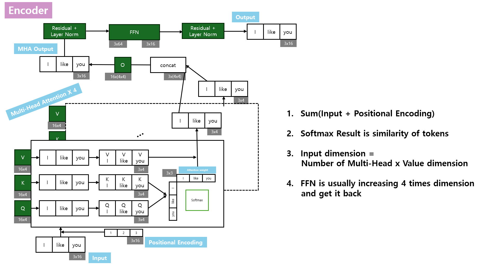
$Transformer\; Block$

$Self-Attention$
How to work on self-attention
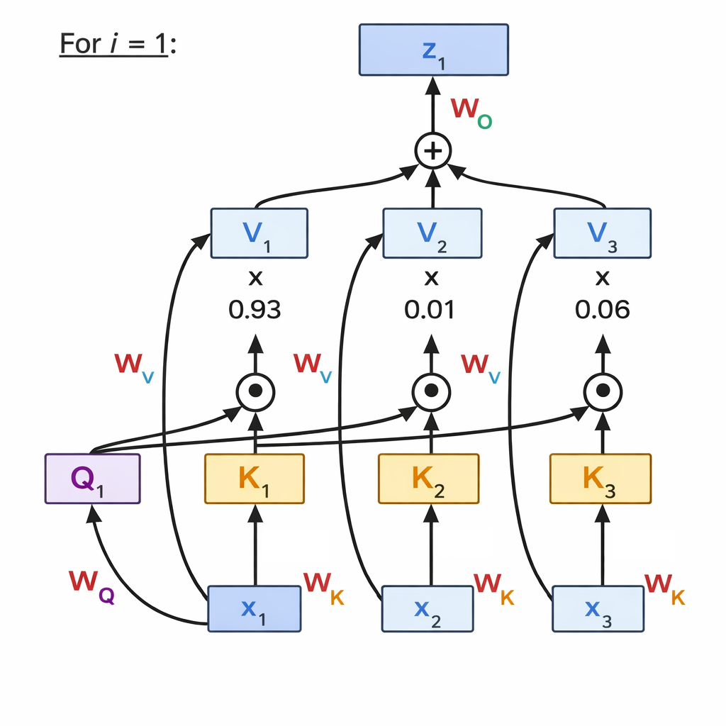
All of the i have same procedure. Transforming from x to z is changing from just token embedding to contextualized token within sequences.
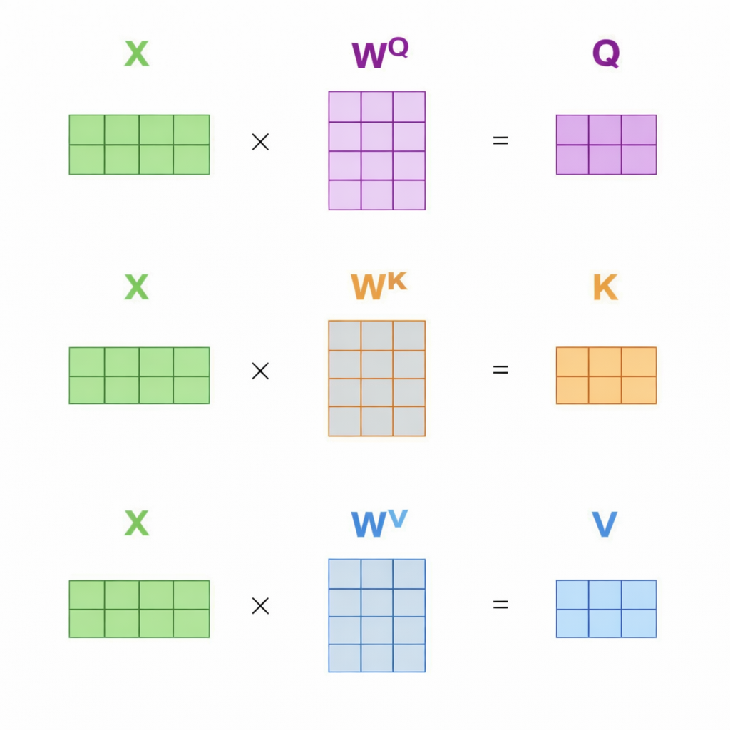
For each input token embedding $x_i \in \mathbb{R}^{d_{\text{model}}}$, we make:
\[q_i = W_Q x_i,\qquad k_i = W_K x_i,\qquad v_i = W_V x_i.\]Where: $ W_Q \in \mathbb{R}^{d_k \times d_{\text{model}}}, \; W_K \in \mathbb{R}^{d_k \times d_{\text{model}}}, \; W_V \in \mathbb{R}^{d_v \times d_{\text{model}}}. $
✅ Same matrices $W_Q,W_K,W_V$ are shared for all tokens.
How to work on self-attention with dimension
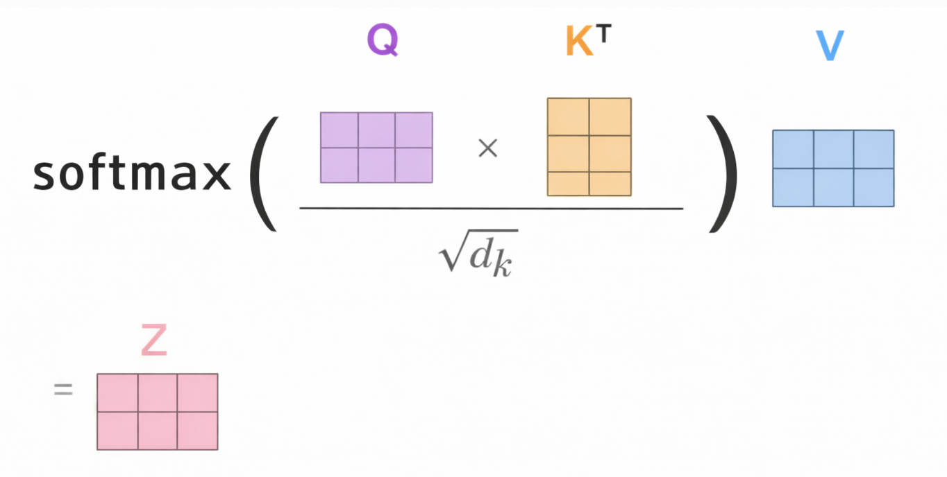
- Self-attention outputs: \(z_i=\sum_j \alpha_{ij}v_j,\quad \alpha_{ij}=\text{softmax}(q_i^\top k_j)\)
Result of Self-Attention Softmax is matrix of similarity between inputs .
Softmax Result is $N$ x $N$ matrix. where: $N$ input size.
Self-Attention main problem is that the mehod ignore the order of tokens.
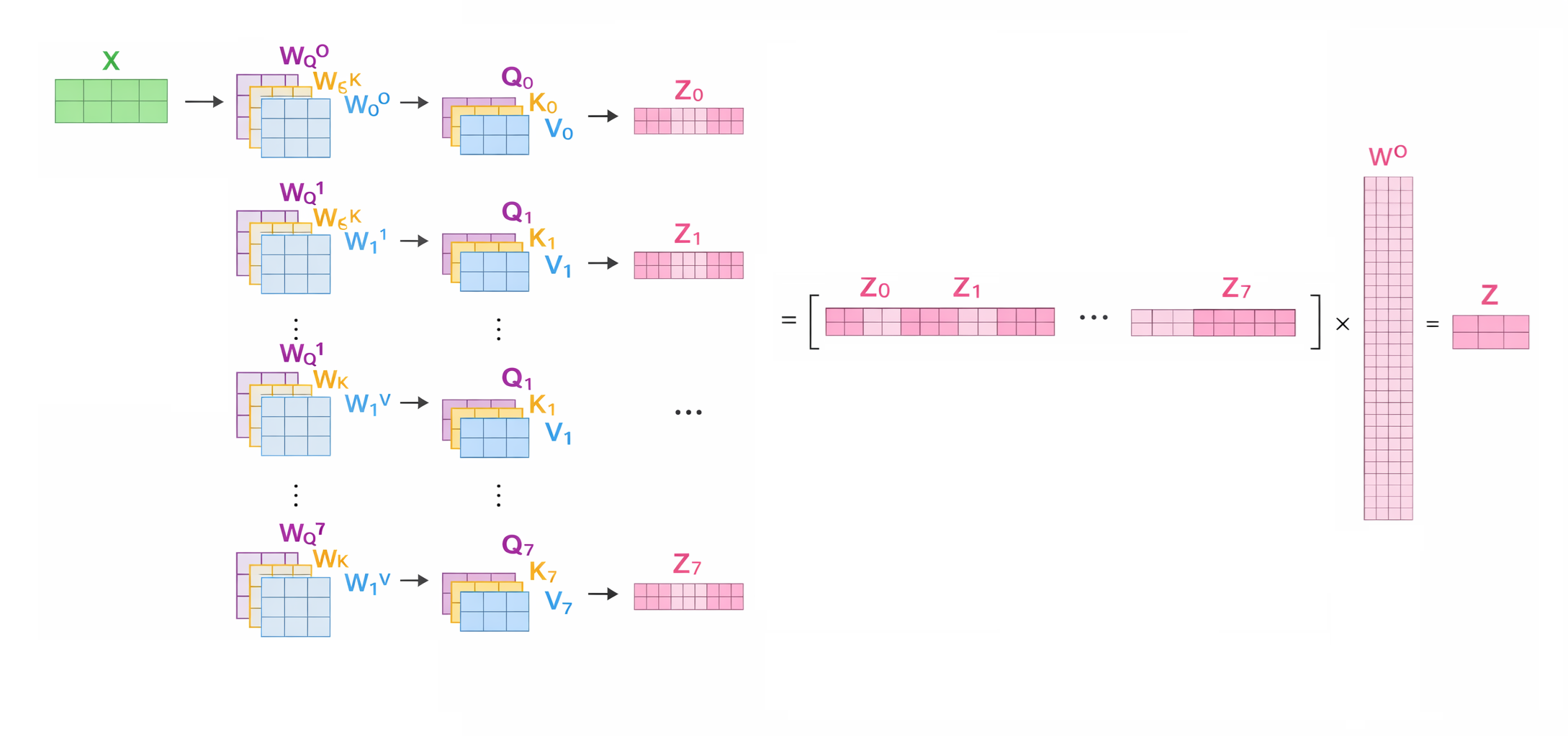
\[MultiHead(Q, K, V) = Concat(head_1, ..., head_h) W_O\]$Multi-Head\; Attention$
\(head_i = Attention(Q W_Q^i, K W_K^i, V W_V^i)\)
$FFN$
Applied independently:
\[\text{FFN}(z) = W_2 \sigma(W_1 z + b_1) + b_2\]where: $ \sigma = \text{ReLU} $
$Residual + LayerNorm$
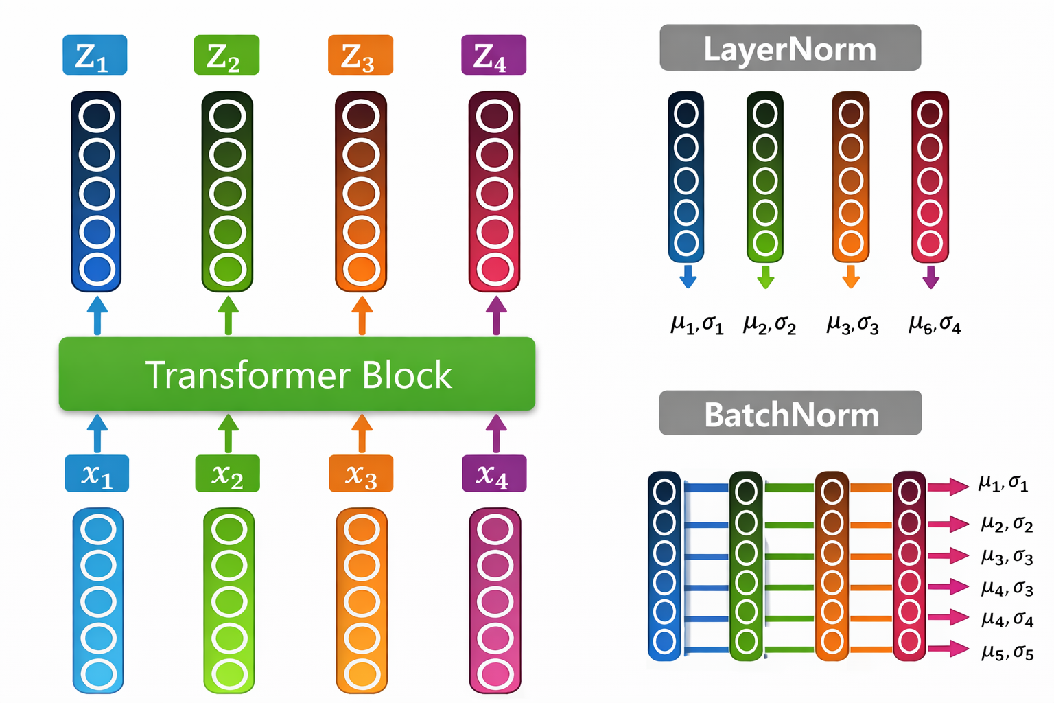
After attention:
\[R' = \text{LayerNorm} \left( R + \text{MultiHead}(R) \right)\]After FFN:
\[R^{\text{next}} = \text{LayerNorm} \left( R' + \text{FFN}(R') \right)\]- Residual helps gradient flow.
- LayerNorm stabilizes scale.
$Positional\; Encoding$
Since attention is permutation invariant, we inject position:
\[r_i = x_i + p_i\]🔷 Sinusoidal Encoding
For $i = 0,\dots,d_{\text{model}}/2 -1$:
\[PE(pos,2i) = \sin\left( \frac{pos}{10000^{2i/d_{\text{model}}}} \right)\] \[PE(pos,2i+1) = \cos\left( \frac{pos}{10000^{2i/d_{\text{model}}}} \right)\]🔎 Why it works (Relative Position Property)
Using identity:
\[\sin(a+b) = \sin a \cos b + \cos a \sin b\]Relative shifts can be represented as linear combinations of sine/cosine pairs.
Thus model can learn relative offsets.
$Stacking\; Blocks$
Repeat above block $L$ times.
Final encoder output:
\[Z^{(L)} \in \mathbb{R}^{N\times d_{\text{model}}}\]Same length as input.
$Masked\; Multi-Head\; Attention$
When we process decoding process, considering the cheating that the i-th input token can not include on the back of the token. So when i-th token is transformed by block, just using 0 ~ (i-1)-th tokens.
With a causal mask, ensuring each token attends only to past and current tokens. Attention weights are computed using masked softmax. It can keep the principle of only using past and current tokens with parallel process.
\[S' = \frac{QK^\top}{\sqrt{d_k}} + M\] \[A = \text{softmax}(S')\]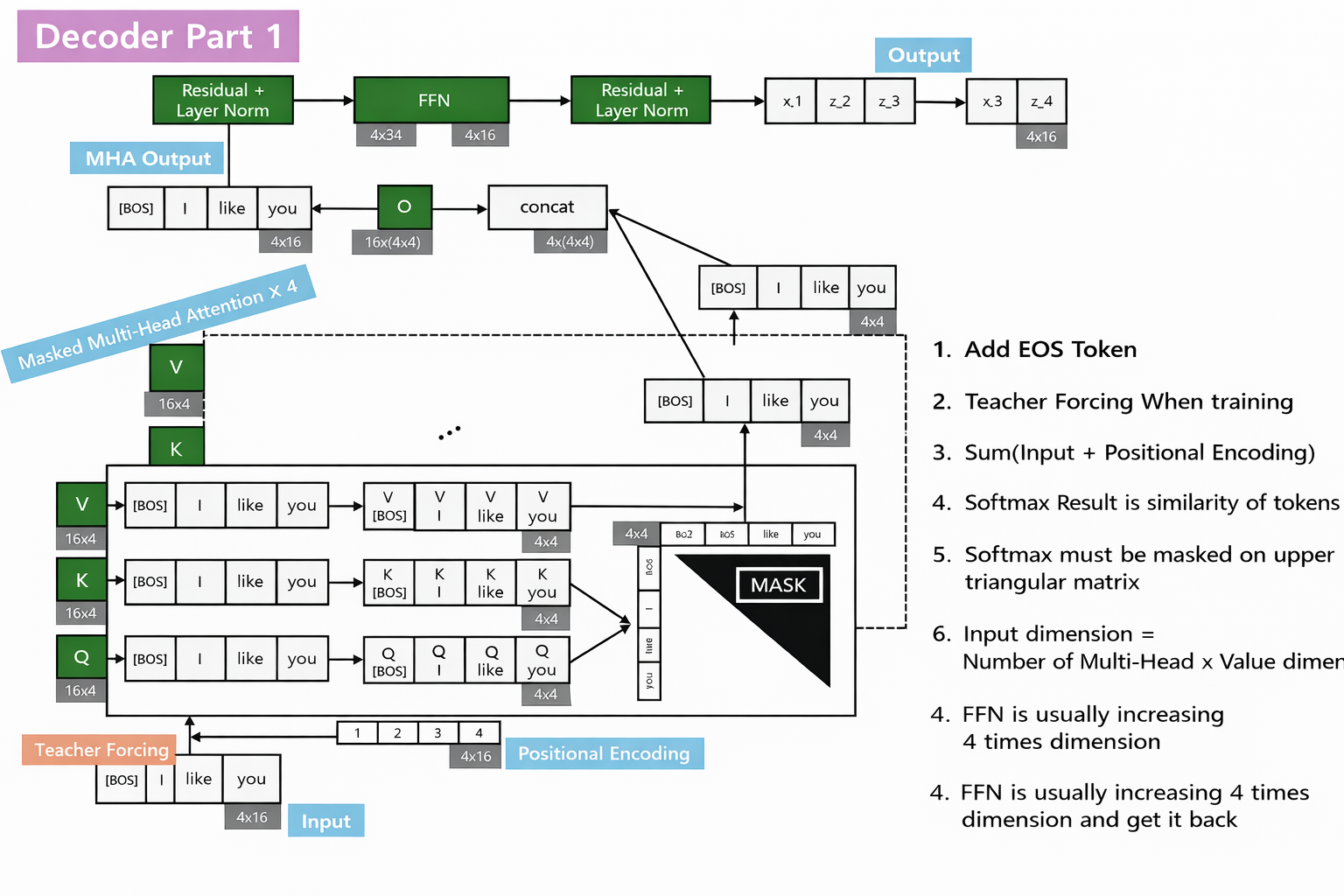
$Encoder-Decoder\; Attention (Cross\; Attention)$
This part is very similiar with encoder transformer block. The only one difference thing is Query input is from decoder previous output, Key Value input is from encoder previous output.
And this part is not needed to use mask on attention weight, because already the output of previous decoder is adapted.
$Decoder\; Queries:$
\[Q = R_{\text{decoder}} W_Q\]$Encoder\; Keys/Values:$
\[K = Z^{(L)} W_K\] \[V = Z^{(L)} W_V\]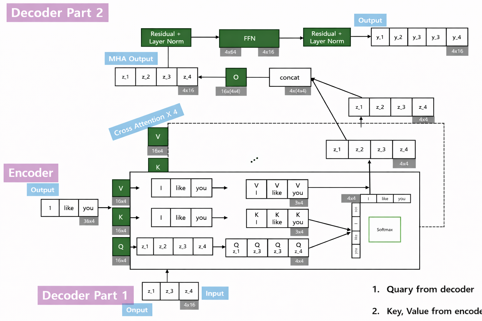
$Linear\; Output\; Layer and SoftMax$
Map to vocabulary logits:
\[o_t = W_o z_t + b_o\] \[W_o \in \mathbb{R}^{|V|\times d_{\text{model}}}\] \[p(y_t=c) = \frac{e^{(o_t)_c}} {\sum_j e^{(o_t)_j}}\]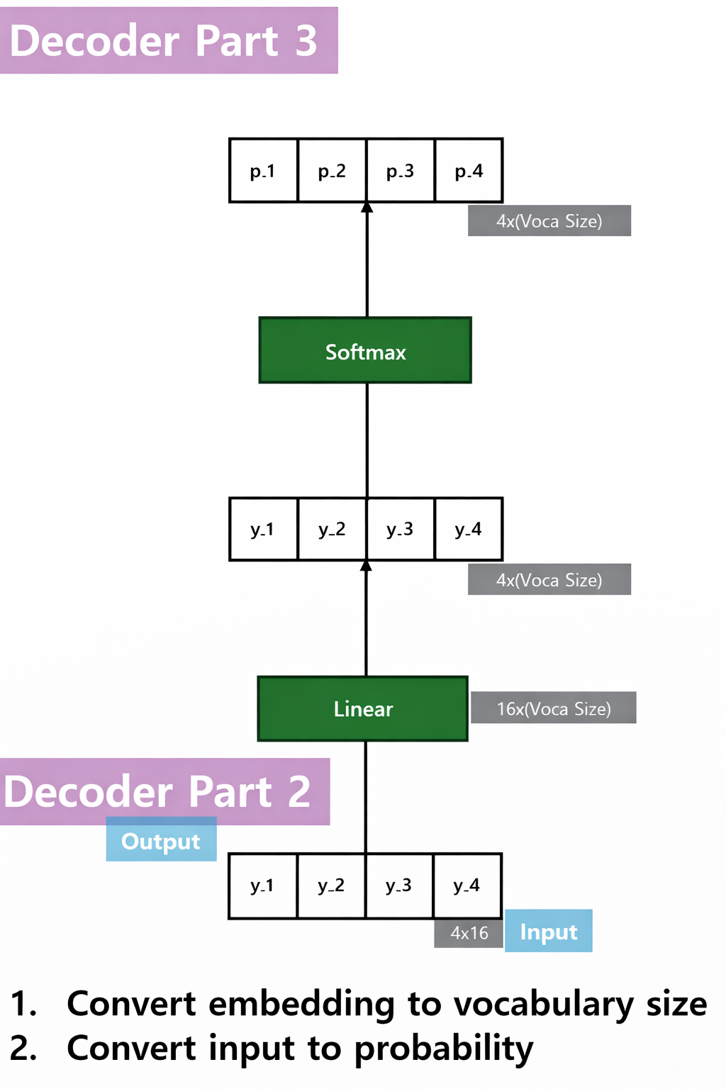
$Cross-Entropy\; Loss\; and\; MLE$
For one-hot target:
\[\mathcal{L}_t = -\sum_c y_{t,c} \log p(y_t=c)\]Sequence loss:
\[\mathcal{L} = \sum_{t=1}^{T} \mathcal{L}_t\] \[P(y_1,\dots,y_T) = \prod_{t=1}^T P(y_t \mid y_{<t}, x)\]Minimize negative log likelihood.
$Inference$
Greedy decoding:
\[\hat{y}_t = \arg\max_c p(y_t=c)\]Beam search keeps top-k sequences.
$Classification\; Variant$
Mean pooling:
\[\bar{z} = \frac{1}{N} \sum_{i=1}^N z_i\]CLS token:
Use:
\[z_{\text{CLS}}^{(L)}\]Extra Information
Why do we scale by ( \sqrt{d_k} ) in Attention?
Problem
Attention scores are computed by: $S = QK^T $
Each score is a dot product of two ( d_k )-dimensional vectors: $ s_{ij} = q_i \cdot k_j $
If vector elements have variance ≈ 1,
then: $\text{Var}(q \cdot k) = d_k, \quad \text{Std} \approx \sqrt{d_k} $
So when ( $d_k$ ) becomes large, attention scores grow large.
Why is this bad?
Softmax is very sensitive to large values.
Example:
$ [20, 5, -3] \xrightarrow{\text{softmax}} [0.999999, \approx 0, \approx 0] $
This makes the distribution almost one-hot, which causes:
- Gradient ≈ 0 (vanishing)
- Slow or unstable learning
- Softmax saturation
Solution: Scale by ( \sqrt{d_k} )
Transformer uses:
$ \text{Attention}(Q,K,V) = \text{softmax}\left(\frac{QK^T}{\sqrt{d_k}}\right)V $
Since:
$ \text{Std}(QK^T) \approx \sqrt{d_k} $
Dividing by $ \sqrt{d_k} $ keeps the variance ≈ 1, preventing scores from becoming too large.
Intuition
- Higher dimension → larger dot product naturally
- Large scores → softmax becomes too sharp
- Sharp softmax → gradients vanish
- Scaling keeps softmax in a stable, non-saturated region
$ \boxed{ \text{Scaling by } \sqrt{d_k} \text{ stabilizes softmax and prevents vanishing gradients.} } $