Why Pattern Matching Scores Cluster

🎯 Practical Observation
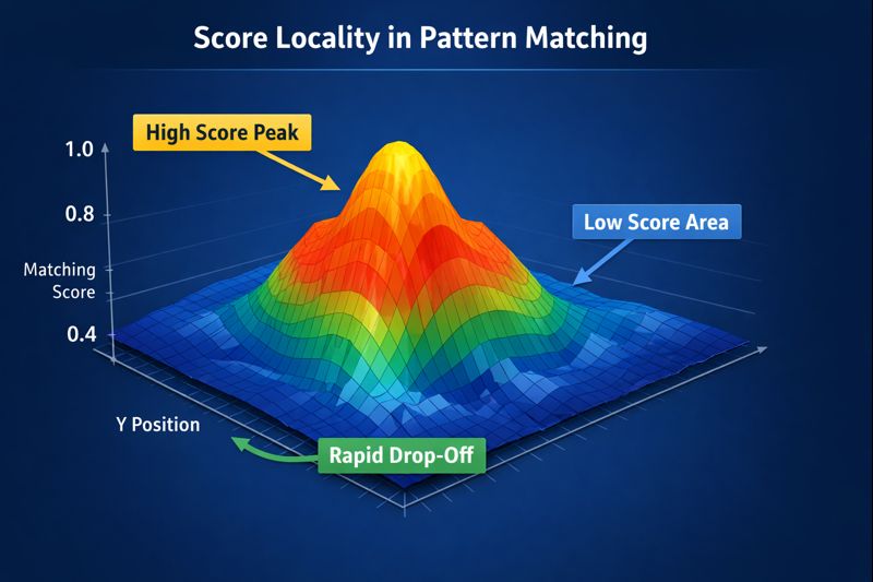
Implement a pattern matcher and you’ll notice something striking:

Scores explode near the correct location — and collapse almost everywhere else.

This is not coincidence. It reflects a core computer vision property.

---

🧠 The Phenomenon: Score Clustering

In real-world pattern matching, score maps rarely look smooth or evenly distributed.

Instead, they show:

• 🔺 One dominant peak
• 📉 Rapid decay away from the peak
• 🟦 Vast background regions with low or near-zero scores

This behaviour is best described as score locality.

---

📍 What Does “Locality” Mean in CV?

In computer vision terms, locality means:

Matching confidence is concentrated within a small spatial neighbourhood.

Concretely:

• Small spatial shifts → small score changes
• Larger misalignments → sudden score collapse

The score map forms a concentrated energy landscape, not random noise.

---

🗺️ Visual Intuition (Score Map)

Low   Low   Low   Low   Low
Low   Low   High  Low   Low
Low   High  MAX   High  Low
Low   Low   High  Low   Low
Low   Low   Low   Low   Low

🔴 The correct match appears as a sharp local maximum, not a wide plateau.

---

🔎 Why Does This Happen? (Vision Interpretation)

🧩 1. Structural Overlap

Most matchers measure structural agreement:

• intensity alignment
• gradient consistency
• edge or shape overlap

Near the correct position:

• Structures still overlap
• Scores remain high

Farther away:

• Overlap breaks rapidly
• Scores drop off a cliff

---

📐 2. Correlation Is Naturally Peaked

Many classical vision matchers rely on correlation-like operations:

• cross-correlation
• normalised cross-correlation
• dot products in feature space

📌 Correlation is inherently peaked when signals align — a mathematical property, not a tuning artefact.

---

🌌 3. High-Dimensional Feature Separation

In feature-based matching:

• Each location maps to a high-dimensional vector
• The correct match lies close to the template vector
• Most background locations are far away

In high dimensions:

• Good matches stand out dramatically
• Background collapses into uniformly low scores

---

⚙️ Engineering Consequences

Understanding score locality directly informs system design.

🚀 Early Rejection

Because most locations are clearly wrong:

• Cheap tests reject them early
• Expensive scoring runs only locally

This enables cascade-style matchers.

---

🪜 Coarse-to-Fine Search

Locality makes hierarchical strategies effective:

1️⃣ Coarse scan
2️⃣ Detect promising regions
3️⃣ Refine locally

This avoids full-resolution brute-force evaluation.

---

⏱️ Stable Runtime

Localised peaks imply:

• Predictable candidate counts
• Low runtime variance

Critical for real-time and industrial systems.

---

✂️ Relation to Non-Maximum Suppression (NMS)

NMS relies on locality:

• Keep the strongest response
• Suppress neighbouring ones

Without score locality, NMS would be unreliable.

---

⚠️ When Locality Weakens

Locality degrades when:

• Patterns are repetitive or symmetric
• Background contains similar structures
• Noise dominates signal

In such cases:

• Multiple peaks emerge
• Additional constraints become necessary

---

💡 A Computer Vision Takeaway

Pattern matching outputs are structured landscapes, not random fields.

Thinking in terms of:

• energy distributions
• local maxima
• spatial confidence

is a computer-vision mindset, not just an algorithm trick.

---

✅ Summary

• 🔹 Pattern matching scores cluster spatially
• 🔹 This reflects score locality
• 🔹 Locality explains why NMS, early rejection, and coarse-to-fine search work
• 🔹 Interpreting score maps leads to better system-level design

---

✨ Seeing the structure behind algorithm outputs is what turns code into engineering.